Neural Style Transfer

Merging a content image and a style image to produce art!

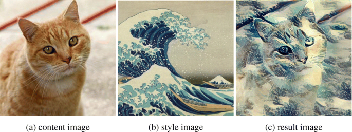
Neural Style Transfer (NST) is an interesting optimization technique in deep learning. It merges to images: a “content” image (C) and a “style” image (S), to create a “generated” image (G).

NST uses a previously trained convolutional network, and builds on top of that. This is called transfer learning. In this project, I will be using the VGG network from the original NST paper. Specifically, I will be using the VGG-19 network, a 19-layer version of the network. This model has been trained on the ImageNet dataset.

1. Style Cost Function

Firstly, to compute the “style” cost, we need to calculate the Gram matrix. This matrix gives us an idea of how similar two feature maps are. The code to compute the Gram matrix is given below. It is just the dot product of the input vectors. We are interested in similarity since we want the style of the Style image and the Generated image to the similar.

Next, once we have the Gram matrices calculated for the Style image and the Generated image, a squared difference can be taken with a normalization constant to obtain the Style loss for a particular layer.

Code

 1
 2
 3
 4
 5
 6
 7
 8
 9
10
11
12
13
14
15
16
17

    def gram_matrix(A):
        GA = tf.matmul(A, tf.transpose(A))
        return GA

    def compute_layer_style_cost(a_S, a_G):

        _, n_H, n_W, n_C = a_G.get_shape()

        a_S = tf.transpose(tf.reshape(a_S, shape=[-1, n_C]))
        a_G = tf.transpose(tf.reshape(a_G, shape=[-1, n_C]))

        GS = gram_matrix(a_S)
        GG = gram_matrix(a_G)

        J_style_layer = tf.reduce_sum(tf.square(tf.subtract(GS, GG)), axis=None)/((2 * n_W * n_H * n_C) ** 2)

        return J_style_layer

2. Content Cost Function

In the shallower layers of a CNN, the model learns low level features whereas in the deeper layers, the model learns complex features. Hence, in the generated image, the content should match that of the input content image. This can be achieved by taking activations from the middle of the CNN.

This cost can be computed by comparing the activations of the style image and the generated image.

Code

 1
 2
 3
 4
 5
 6
 7
 8
 9
10
11
12

    def compute_content_cost(content_output, generated_output):
        a_C = content_output[-1]
        a_G = generated_output[-1]

        m, n_H, n_W, n_C = a_G.get_shape()

        a_C_unrolled = tf.reshape(a_C, shape=[m, -1, n_C])
        a_G_unrolled = tf.reshape(a_G, shape=[m, -1, n_C])

        J_content = tf.reduce_sum(tf.square(tf.subtract(a_G_unrolled, a_G_unrolled)), axis=None)/(4 * n_W * n_C * n_H)

        return J_content

3. Total Cost

The total cost function is just a weighted sum of the Style Cost and the Content Cost.

Code

1
2
3

    @tf.function()
    def total_cost(J_content, J_style, alpha = 10, beta = 40):
        return alpha * J_content + beta * J_style

4. Optimization Loop

The various steps for solving the optimization problem are:

1. Load the content image
2. Load the style image
3. Randomly initialize the image to be generated
4. Load the VGG19 model
5. Compute the content cost
6. Compute the style cost
7. Compute the total cost
8. Define the optimizer and learning rate

The training loop looks like:

Code

 1
 2
 3
 4
 5
 6
 7
 8
 9
10
11
12
13
14
15
16

    optimizer = tf.keras.optimizers.Adam(learning_rate=0.03)

    @tf.function()
    def train_step(generated_image):
        with tf.GradientTape() as tape:
            a_G = vgg_model_outputs(generated_image)
            J_style = compute_style_cost(a_S, a_G)
            J_content = compute_content_cost(a_C, a_G)
            J = total_cost(J_content, J_style, alpha=20, beta=40)

        grad = tape.gradient(J, generated_image)

        optimizer.apply_gradients([(grad, generated_image)])
        generated_image.assign(clip_0_1(generated_image))

        return J