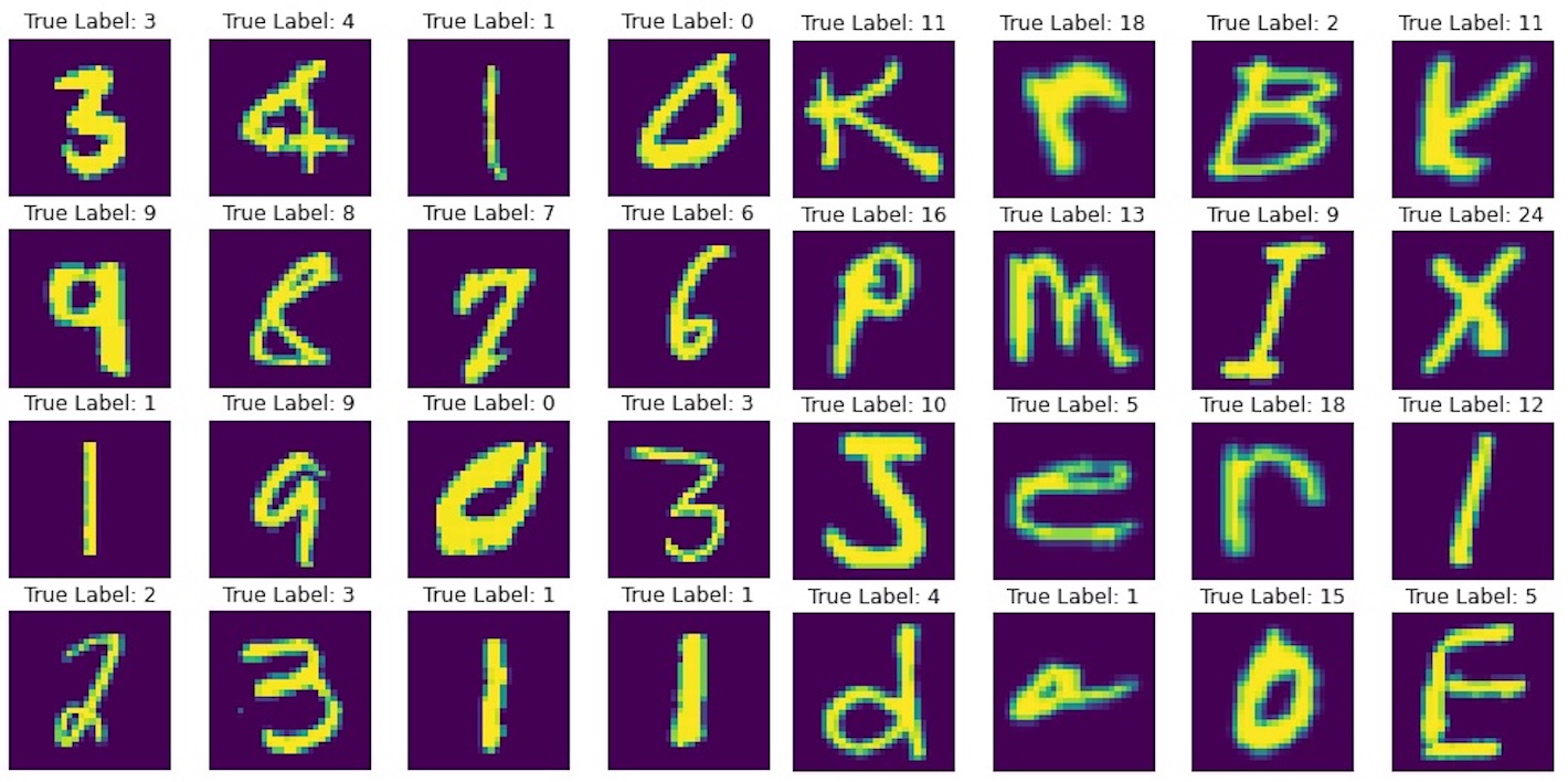
Building a handwritten digits and characters classifier from scratch.
The goal of this project was to understand the inner workings of a Neural Network by coding the initialization, learning and testing algorithms from scratch using the NumPy library.
1. The Dataset
- MNIST:
- This is the well known handwritten digits dataset that is the “Hello World” of Computer Vision. It consists of images of digits (0-9) written by hand, each of size 28x28 pixels.
- MNIST:
- This is the handwritten characters dataset that contains images of both lower and upper case characters. Similar to the MNIST dataset, each image is of size 28x28 pixels.
The images in these datasets were visualized using
matplotlib.
Code
1
2
3
4
5
6
7
8
9
|
    sprint("Sample of images from the MNIST Dataset : ")
    plt.figure(figsize=(8, 8))
    for i in range(16):
        plt.subplot(4, 4, i+1)
        plt.axis('off')
        r = np.random.randint(x_train.shape[0])   ## PICK A RANDON IMAGE TO SHOW
        plt.title('True Label: '+ str(y_train[r])) ## PRINT LABEL
        plt.imshow(x_train[r].reshape(28, 28))     ## PRINT IMAGE
    plt.show()
|
2. The N-layer Feed Forward Neural Network
Initializing Parameters for all layers
 1
 2
 3
 4
 5
 6
 7
 8
 9
10
11
12
13
14
15
16
17
|
    # dim( W[l] ) = ( n[l], n[l-1] )
    # dim( b[l] ) = ( 1, n[l] )
    # where,
    #   l = current layer
    #   W[l] = weights of current layer
    #   b[l] = bias for the current layer
    #   n[l] = number of nodes in current layer

    def initialize_parameters(layer_dims):
    parameters = {}
    L = len(layer_dims)

    for i in range(1, L):
        parameters['W' + str(i)] = np.random.randn(layer_dims[i], layer_dims[i-1])*0.01
        parameters['b' + str(i)] = np.zeros((1, layer_dims[i])) + 0.01

    return parameters
|
Forward and Backward Propagation
 1
 2
 3
 4
 5
 6
 7
 8
 9
10
11
12
13
14
15
16
17
18
19
20
21
22
23
24
25
26
27
28
29
30
31
32
33
34
35
36
37
38
39
40
41
42
43
44
45
46
47
48
49
50
51
52
53
54
55
56
57
58
59
60
61
62
63
64
65
|
    # Forward propagation equations:

    # Z[l] = W[l].X + b[l]
    # A[l] = g( Z[l] )
    # Where,
    #     Z = weighted sum of input and bias
    #     A = activations of particular layer
    #     l = layer

    # Backward propagation equations:

    # Err(j)(output layer) = O(j)(1 - O(j))(T(j) - O(j))
    # Err(j)(hidden layer) = O(j)(1 - O(j))(SUM(Err(k)W(j,k)
    # del(W(i,j)) = (l)Err(j)O(i)
    # del(b(j)) = (l)Err(j)
    # Where,
    #       O: Output of a node
    #       W: weight
    #       b: bias
    #       i, j, k: nodes

    def sigmoid(X):
        return 1/(1 + np.exp(-1*X))

    def forward_step(A_prev, W, b):
        return sigmoid(np.dot(A_prev, W.T) + b)

    def computation_n(X, y, parameters, eta, num_iters):
        hidden_output = []
        hidden_error = []
        m = X.shape[0]
        L = (len(parameters)//2) + 1      # number of layers

        # iterating for given number of iterations
        for itr in range(num_iters):
            # for each training example
            for i in range(m):
                # forward propagation for n layers
                hidden_output.append(X[i])
                A_prev = X[i]
                for l in range(1, L):
                    A_prev = forward_step(A_prev, parameters['W' + str(l)], parameters['b' + str(l)])
                    hidden_output.append(A_prev)

                # propagating the error backwards
                # print('hidden_output[-1].shape: {}; y[i].shape: {}'.format(hidden_output[-1].shape, y[i].shape))
                dOutput = hidden_output[-1]*(1 - hidden_output[-1])*(y[i] - hidden_output[-1])
                hidden_error.append(dOutput)
                k = 0
                for l in reversed(range(1, L-1)):
                    error = hidden_output[l]*(1 - hidden_output[l])*np.dot(hidden_error[k], parameters['W' + str(l+1)])
                    hidden_error.append(error)
                    k += 1

                # parameter changes
                k = 0
                for l in reversed(range(1, L)):
                    parameters['W' + str(l)] += eta*hidden_error[k].reshape(-1, 1)*hidden_output[l-1]
                    parameters['b' + str(l)] += eta*hidden_error[k]
                    k += 1

                hidden_output.clear()
                hidden_error.clear()

        return parameters
|
3. Training and Testing
The MNIST and EMNIST datasets were loaded and the labels were One-Hot encoded. The parameters for the models were initialzed and the model was trained on the training split obtained by using the train_test_split method imported from sklearn.model_selection. Furthermore, the pixel values were normalized to the range [0-1] for more efficient computation. The results are shown below:
Code
 1
 2
 3
 4
 5
 6
 7
 8
 9
10
11
12
13
14
15
16
17
18
19
20
21
22
23
24
25
26
27
28
29
30
31
|
    # Handwritten digits classification
    parameters = initialize_parameters([784, 50, 50, 10])
    print("Length of parameters dictionary : {}".format(len(parameters)))
    Length of parameters dictionary : 6

    print("Training model...")
    parameters = train(x_train, y_train, parameters, 0.01, 20)
    Training model...

    print("Testing model...")
    print('Training error : ', end='')
    test(x_train, y_train, parameters)
    print('\nTesting error : ', end='')
    test(x_test, y_test, parameters)
    Testing model...
    Training error : Accuracy : 98.791 %
    Testing error : Accuracy : 98.772 %

    # Handwritten characters classification
    parameters = initialize_parameters([784, 50, 50, 27])
    print("Length of parameters dictionary : {}".format(len(parameters)))
    Length of parameters dictionary : 6

    print("Training model...")
    parameters = train(X_train, y_train, parameters, 0.01, 20)
    Training model...

    print("Testing model...")
    test(X_test, y_test, parameters)
    Testing model...
    Accuracy : 96.29629629629629 %
|
4. Results
By coding a Neural Network from scratch, I was able to get a better understanding of the math behind the magic.
